Adhesive CZM ANSYS Parameters
Motivation
Perhaps one of the biggest curse to any engineering analyst is the the lack of key parameters to make a good estimate. For adhesive modeling, what parameters should one use? One can try to look up typical values online or from research papers but they are often not exactly what's being used immediately.
To overcome this difficulty, you could create an experimental test for your adhesive to extract the information you need as described in the paper by Dastjerdi et al [1].
The rest of the blog post details how to interpret the test data. Next, by using extracted parameters, replicate the test in Ansys to get similar results (as expected).
A few years ago, I was pulled in to do some adhesive modeling. The project leaders later decided against using adhesives but it peaked my interest on how to simulate adhesives using Cohesive Zone Modeling (CZM). Mode I Peel direction failure was a concern and glue manufacturers sometimes lists the peel strength per ASTM D 1876. Unfortunately, from those values alone, it is difficult to determine the needed parameters for use in ANSYS.
Simulation Model Goal
Unlike ASTM D1876, the paper by Dastjerdi et al [1] provides a clear way of translating load frame test data into parameters used in ANSYS. The flimsy panels used in the ASTM standard are highly non-linear. The critical contribution of the paper is to replace highly deformable test pieces with a rigid body substrate and providing the math in computing the parameters.

Figure 1: Fixtures used in CZM Adhesive Characterization
The second piece of the puzzle is SR #2052789 which provides many tips on the model setup requirements (e.g. Never update contact stiffness, use fracture object etc). Their attached project file was used as a template for this blog post's project.
The paper by Dastjerdi et al [1] shows how one could calculate the normal traction vs separation from their experimental setup. The experimental setup and corresponding test results were also described well enough to be replicated in ANSYS. As both test data and calculated cohesive laws curve are available in the paper, we could extract CZM CBDD parameters then try to replicate the test in ANSYS to see how well the calculated force measures up to test data. This would be done for the Polyurethane adhesive.
Extracting Parameters from Test Data
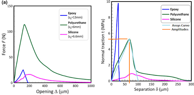
Figure 7 & 8 from the paper shows the measured force vs opening and normal traction vs separation respectively. Please see the paper on how to compute the nominal traction vs separation plot.
Next, I appended in Figure 2 below, the light turquoise line was appended over the green Polyurethane line to approximate the ANSYS load path. The vertical and horizontal appended orange lines helps determine the amplitudes for this path (5.2MPa & 70micro-meter).
The CZM Separation-Distance Debonding parameters approximated from the turquoise line are:

Note the peak normal traction stress is used in Fig 3. A key snippet is needed for the initial gradient which specifies the stiffness of the contact elements:

Figure 2: Appended Plots from Paper
The CZM Separation-Distance Debonding parameters approximated from the turquoise line are:

Figure 3: CZM Properties
Note the peak normal traction stress is used in Fig 3. A key snippet is needed for the initial gradient which specifies the stiffness of the contact elements:
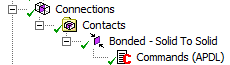
Figure 4: Stiffness Specification Location
The snippet is:
rmod,cid,3, -0.07428e12 ! FKN = 5.2e6/70e-6
rmod,cid,11,-0.07428e12 ! FKOP = 5.2e6/70e-6
Note both the peak stress and separation is included in the above snippet. The negative value tells Ansys to interpret the real constants FKN & FKOP as absolute value and not based on the underlying element stiffness/dimensions. Other details can be found in the archived model.
Results & Discussion
Figure 5 has the calculated force peaks at 97.5N at 0.12mm opening.

It's a bit smaller than the peak ~112N at ~0.14mm shown in the paper but it's not far in the left field. A bit more parameter tweaking should better match the ANSYS results to the test forces.
Note that a shear test (Mode II) is advised to determine the tangential properties which were (wrongly) assumed to be the same in the above example.
Figure 5: Calculated Force
It's a bit smaller than the peak ~112N at ~0.14mm shown in the paper but it's not far in the left field. A bit more parameter tweaking should better match the ANSYS results to the test forces.
Note that a shear test (Mode II) is advised to determine the tangential properties which were (wrongly) assumed to be the same in the above example.
Key Resources
1. CAEAI presentation [link] provides good background information
2. PADT The Focus #56 by Rod Scholl [link] explained the parameters clearly
3. Paper by A. Khayer Dastjerdi & E. Tan & F. Barthelat [link] or [link]
4. Ansys Knowledge Resource #2052789 [link] model with bonded contacts
Archive File
ANSYS WB v18.2 [Link]
[1] Khayer Dastjerdi, A., Tan, E. & Barthelat, F. Direct Measurement of the Cohesive Law of Adhesives Using a Rigid Double Cantilever Beam Technique. Exp Mech 53, 1763–1772 (2013). https://doi.org/10.1007/s11340-013-9755-0
Thank you very very very much, It was the only single explanations of many confusions. Just a small question why two commands FKN and FKOP is needed? And what is 3 & 11? Can you please tell.
ReplyDeleteHi Puhan,
DeleteFKN and FKOP is needed as it defines the contact's normal contact stiffness and opening stiffness respectively. Secondly, the real constants of FKN and FKOP corresponds to 3 and 11 respectively. Please see the help of RMODIF and CONTA171 for further details. Good luck!
Your this article is so helpful to me as I try to CZM analysis for DCB and single lap adhesively joints, I appreciate it. However, I have a problem.
ReplyDeleteAs you can see in his paper below, he obtained result about 9kN when the lap length is 25 mm (reference Fig. 8). On the other hand, my result is approximate 600N. I don't know the causes.
I refer to araldite 2015 (Table 1) for analysis.
He used Abaqus, but I use Ansys mechanical for 2D analysis.
could you give me any advice?
in the end, can we define trapezoidal shape in Ansys?
https://doi.org/10.1016/j.proeng.2015.08.047
It's hard to troubleshoot your problem without having a closer look. Perhaps try recreating Fig 7 in the reference paper. Being mostly in sheer, some rough hand calculation is possible. Hopefully that provides some insight on where to look for the problem.
DeleteThis article helps a lot. I have a question for now. How did you find the artificial damping coefficient?
ReplyDeleteArtificial damping is to aid convergence iteration of the nonlinear equations and is arbitrarily set. Please see https://www.mm.bme.hu/~gyebro/files/ans_help_v182/ans_thry/thy_mat11.html. You may start out with a small value and increase it if necessary.
Deletecan we use FKT and FKOP to define a tangential crack propagation stiffness? Also how to can we know the contact id's from our geometry? like in the snippet cid 3 and cid 11 referes to what exactly? please guide. Thank you
ReplyDeleteFor the Debonding Interface mode, I use Mode II. And, I also want to define the tangential stiffness Please do you know what apdl command can be used ?
ReplyDeleteYou may take a look at real constant 12 (FKT) Tangent penalty stiffness factor. Also look at values in Fig 3 you may consider changing.
Delete